Impact of dataset imbalance on QML algorithms

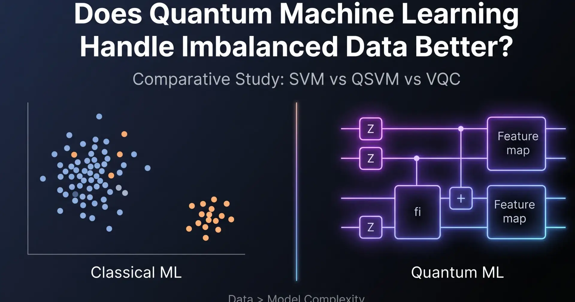
I started this project with a very specific question in mind. Quantum machine learning is often described as a more expressive, more powerful extension of classical learning. If that’s true, does it actually help when the data itself is messy?

More precisely, does it behave differently when the dataset is imbalanced?

That question sounds simple, but it sits at the intersection of two things people usually study separately: model capability and data quality. Most research focuses on improving models. Very little examines how those models behave when the input data is flawed in predictable ways.

Class imbalance is one of the simplest ways to test that.

Why class imbalance is a structural problem

In a binary classification setting, class imbalance means the empirical distribution of labels is skewed. One class appears more frequently than the other.

Suppose 90 percent of the dataset belongs to class 0 and 10 percent to class 1. A classifier trained with standard empirical risk minimization will naturally minimize loss by predicting class 0 most of the time. This is not a bug. It is the expected outcome of the objective function.

From a statistical perspective, the model is optimizing for the observed distribution, not the underlying reality.

The problem shows up immediately in evaluation. Accuracy becomes dominated by class frequency. A trivial classifier that always predicts the majority class achieves 90 percent accuracy without learning anything about the minority class.

This is why recall and F1 score matter more in imbalanced settings. They measure whether the model is actually identifying the minority class.

To isolate the effect of imbalance, I created controlled datasets with fixed feature distributions and varying class priors:

50:50 - 60:40 - 70:30 - 80:20 - 90:10

The geometry of the data stays the same. Only the class distribution changes.

This setup ensures that any performance change comes from imbalance, not from differences in feature space.

Quantum machine learning in practical terms

Quantum machine learning changes how data is embedded and compared.

In a classical model like SVM, the kernel function defines similarity between data points. In a quantum model, data is encoded into quantum states using a feature map. Similarity becomes the overlap between those states.

For a quantum kernel, this looks like:

K(xᵢ, xⱼ) = |⟨φ(xᵢ) | φ(xⱼ)⟩|²

This implicitly maps the data into a high-dimensional Hilbert space. The hope is that complex patterns become linearly separable in that space.

In this project, I used two quantum approaches:

QSVM, which replaces the classical kernel with a quantum kernel

VQC, which uses a parameterized quantum circuit and learns parameters through classical optimization

To anchor the comparison, I used a classical SVM with an RBF kernel.

All models were trained on the same datasets, using the same preprocessing and evaluation metrics.

The quantum models were implemented using Qiskit in a simulated environment, which reflects current NISQ constraints.

Making the task non-trivial

The Iris dataset, even in binary form, is almost linearly separable. If you train directly on it, most models achieve near-perfect performance. That does not reveal meaningful differences.

To create a more realistic setting, I modified the dataset in three ways.

First, I reduced the feature space to two dimensions. This aligns with the limited number of qubits available in small circuits.

Second, I added Gaussian noise after scaling:

X′ = X_scaled + N(0, σ²)

This introduces overlap between classes and removes clean boundaries.

Third, I introduced a nonlinear interaction term by multiplying the two features. This forces the model to learn a nonlinear decision boundary.

After these transformations, the dataset contains overlapping regions. Classification becomes ambiguous, which is where model behavior becomes informative.

Behavior of classical SVM under imbalance

The classical SVM establishes the baseline.

At a balanced ratio, the model performs as expected. It separates the classes with a reasonable margin, and both precision and recall remain stable.

As the imbalance increases, the behavior shifts in a predictable way.

Accuracy increases because the model predicts the majority class more often. Recall for the minority class decreases because fewer minority samples influence the decision boundary. F1 score drops as a result.

At higher imbalance levels, the model converges to a degenerate solution. It predicts the majority class almost exclusively.

This is not random failure. It is the direct consequence of optimizing hinge loss under skewed class distributions.

What the confusion matrix shows

The confusion matrix makes the failure mode explicit.

At extreme imbalance:

True positives for the minority class approach zero .False negatives dominate .Predictions collapse to a single class

The model has learned a shortcut that minimizes loss. It has not learned the minority class.

QSVM: different representation, same outcome

QSVM changes the feature space through a quantum kernel. In principle, this could allow better separation of complex patterns.

However, imbalance is not purely a geometric issue. It is also a sampling issue.

The kernel matrix reflects pairwise similarities between samples. When minority samples are underrepresented, their influence on the optimization problem is reduced. The decision boundary still shifts toward the majority class.

Empirically, QSVM follows the same trend as classical SVM. Accuracy increases with imbalance. Recall and F1 score decrease. At higher imbalance levels, the model fails to detect the minority class.

The quantum kernel changes how data is represented. It does not change how often each class appears.

VQC: optimization under constrained information

VQC introduces a different learning mechanism. Instead of relying on a fixed kernel, it learns parameters in a quantum circuit.

This adds flexibility, but it also introduces new challenges.

The optimization process depends on gradients derived from measurement outcomes. Under imbalance, the contribution of minority samples to the loss function becomes small. The optimizer receives weaker signals about that class.

At the same time, the circuit is shallow and noisy, and the parameter space can contain flat regions. This makes convergence unstable.

The observed behavior reflects these constraints:

Higher variance across runs, Lower stability ,Performance degradation even at moderate imbalance

The model does not simply mimic SVM. It fails for different reasons, but it still fails.

Comparative analysis across models

Plotting all three models on the same axis clarifies the dominant pattern

SVM and QSVM show similar degradation curves. VQC shows more variability but follows the same overall trend. As imbalance increases, minority class performance collapses.

The differences between models are secondary. The class distribution drives the outcome.

What actually changes, and what does not

Quantum models change the embedding of data and the mechanism of learning. They do not change the empirical distribution of the dataset.

If the dataset underrepresents a class, the model receives less information about that class. This affects both classical and quantum models in the same way.

QSVM demonstrates that a richer feature space does not compensate for skewed sampling. VQC shows that adding trainable parameters does not solve the problem either.

The limitation is not in representation. It is in the data.

Implications for quantum machine learning

These results point to a simple conclusion.

Improving the model alone is not enough.

Handling imbalance requires explicit intervention:

Reweighting the loss function

Oversampling or undersampling

Using metrics that penalize imbalance during training

Without these, even highly expressive models converge to biased solutions.

Quantum models do not bypass this requirement. They inherit it.

Closing observation

The original question was whether quantum machine learning models handle imbalanced data better.

They do not.

The experiments show that class imbalance affects all models in similar ways. Accuracy can increase while meaningful performance decreases. Minority class detection collapses as imbalance grows.

The constraint comes from the data distribution, not from the model class.

Better models do not fix bad data. They learn its bias.