📘 Linear Regression and Beyond: A Deep Dive into Core ML Concepts

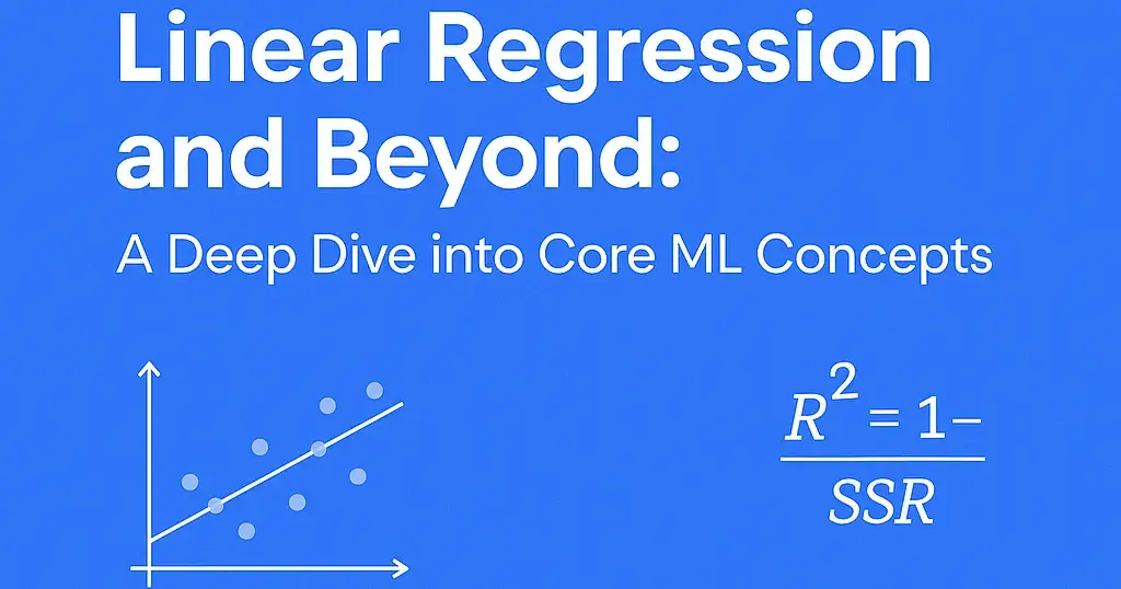
Machine Learning begins with understanding how we can make predictions based on data. One of the most fundamental algorithms to start with is Linear Regression. This article walks you through Linear Regression, the math behind it, gradient descent, model evaluation, and much more — perfect for both beginners and intermediate ML enthusiasts.

🔹 1. Linear Regression

Linear Regression is a supervised learning algorithm used for predicting a continuous dependent variable based on one or more independent variables.

Simple Linear Regression Equation:

y=mx+c

Where:

• y is the dependent variable (output)

• x is the independent variable (input)

• m is the slope (coefficient)

• c is the intercept

Example:
Predicting house prices based on area.

from sklearn.linear_model import LinearRegression
model = LinearRegression()
model.fit(X_train, y_train)
predictions = model.predict(X_test)

🔹 2. Mathematical Intuition Behind Linear Regression

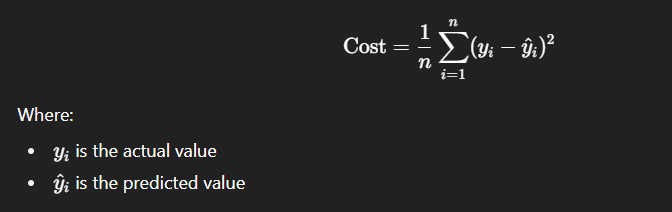
Linear regression finds the best-fitting straight line (regression line) through the data points by minimizing the error between predicted and actual values.

Mathematically, we aim to minimize the Cost Function (Loss Function):

🔹 3. Optimizers in ML

Optimizers are algorithms used to minimize the loss function by updating model parameters (weights and biases). Common optimizers include:

• Gradient Descent

• Stochastic Gradient Descent (SGD)

• Adam

• RMSProp

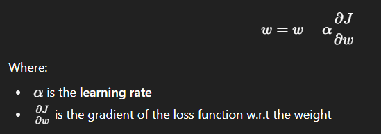
🔹 4. Gradient Descent Algorithm

Gradient Descent is an optimization algorithm that minimizes the cost function by updating weights in the opposite direction of the gradient.

Update Rule:

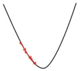
🔹 5. Learning Rate in Gradient Descent

The learning rate (α) determines how big the steps are while reaching the minimum of the loss function.

• Too high → may overshoot the minimum

• Too low → slow convergence

What is Learning Rate?

Learning rate is a important hyperparameter in gradient descent that controls how big or small the steps should be when going downwards in gradient for updating models parameters. It is essential to determines how quickly or slowly the algorithm converges toward minimum of cost function.

1. If Learning rate is too small: The algorithm will take tiny steps during iteration and converge very slowly. This can significantly increases training time and computational cost especially for large datasets.

2. If Learning rate is too big: The algorithm may take huge steps leading overshooting the minimum of cost function without settling. It fail to converge causing the algorithm to oscillate. This process is termed as exploding gradient problem.

Working of Gradient Descent

• Step 1 we first initialize the parameters of the model randomly 

• Step 2 Compute the gradient of the cost function with respect to each parameter. It involves making partial differentiation of cost function with respect to the parameters. 

• Step 3 Update the parameters of the model by taking steps in the opposite direction of the model. Here we choose a hyperparameter learning rate which is denoted by γγ. It helps in deciding the step size of the gradient. 

• Step 4 Repeat steps 2 and 3 iteratively to get the best parameter for the defined model.

Advantages Of Gradient Descent 

• Flexibility: It can be used with various cost functions and can handle non-linear regression problems.

• Scalability: It is scalable to large datasets since it updates the parameters for each training example one at a time.

• Convergence: It can converge to global minimum of the cost function provided that the learning rate is set appropriately.

Disadvantages Of Gradient Descent 

• Sensitivity to Learning Rate: The choice of learning rate is important in gradient descent as it can lead to vanishing or exploding gradient problem.

• Sensitivity to initialization: It can be sensitive to the initialization of the models parameters which can affect the convergence and the quality of the solution.

• Local Minima: It can get stuck in local minima, if the cost function has multiple local minima.

• Time-consuming: It can be time-consuming especially when dealing with large datasets.

Gradient Descent is a fundamental optimization technique used in machine learning. Understanding it allows us to make efficient and accurate model by reducing error made by model using cost function during their training phase, making gradient descent essential for building effective machine learning models.

🔹 6. Loss Function vs Cost Function

• Loss Function: Error for a single observation

• Cost Function: Average of the loss across all data points

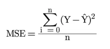
In linear regression, both are typically the Mean Squared Error (MSE).

🔹 7. Assumptions of Linear Regression

1. Linearity

Assumption: The relationship between the independent and dependent variables is linear.

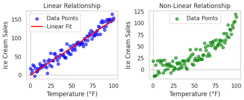
The first and foremost assumption of linear regression is that the relationship between the predictor(s) and the response variable is linear. This means that a change in the independent variable results in a proportional change in the dependent variable. This can be visually assessed using scatter plots or residual plots.

If the relationship is not linear, the model may underfit the data, leading to inaccurate predictions. In such cases, transformations of the data or the use of non-linear regression models may be more appropriate.

Example:

Consider a dataset where the relationship between temperature and ice cream sales is being studied. If sales increase non-linearly with temperature (e.g., significantly more sales at high temperatures), a linear model may not capture this effect well. We'll also show a scenario where the relationship is not linear.

• Linear Relationship: This is where the increase in temperature results in a consistent increase in ice cream sales.

• Non-Linear Relationship: In this case, the increase in temperature leads to a more significant increase in ice cream sales at higher temperatures, indicating a non-linear relationship.

2. Independence of Errors

Independence of errors is another critical assumption for linear regression models. It ensures that the residuals (the differences between the observed and predicted values) are not correlated with one another. This means that the error associated with one observation should not influence the error of any other observation. When errors are correlated, it can indicate that some underlying pattern or trend in the data has been overlooked by the model.

If the errors are correlated, it can lead to underestimated standard errors, resulting in overconfident predictions and misleading significance tests. Violation of this assumption is most common in time series data, where the error at one point in time may influence errors at subsequent time points. Such patterns suggest the presence of autocorrelation.

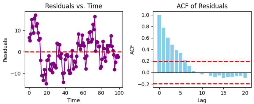
In the Image above,

• The Residuals vs. Time plot: shows a random scatter of points, suggesting no clear pattern or correlation over time.

• The ACF of Residuals plot shows a few spikes at low lags, but they are not significant enough to indicate strong autocorrelation.

3. Normality - Normal Distribution

Multivariate normality is a key assumption for linear regression models when making statistical inferences. Specifically, it means that the residuals (the differences between observed and predicted values) should follow a normal distribution when considering multiple predictors together. This assumption ensures that hypothesis tests, confidence intervals, and p-values are valid.

This assumption is crucial because it allows us to make valid inferences about the model's parameters and the relationship between the dependent and independent variables.

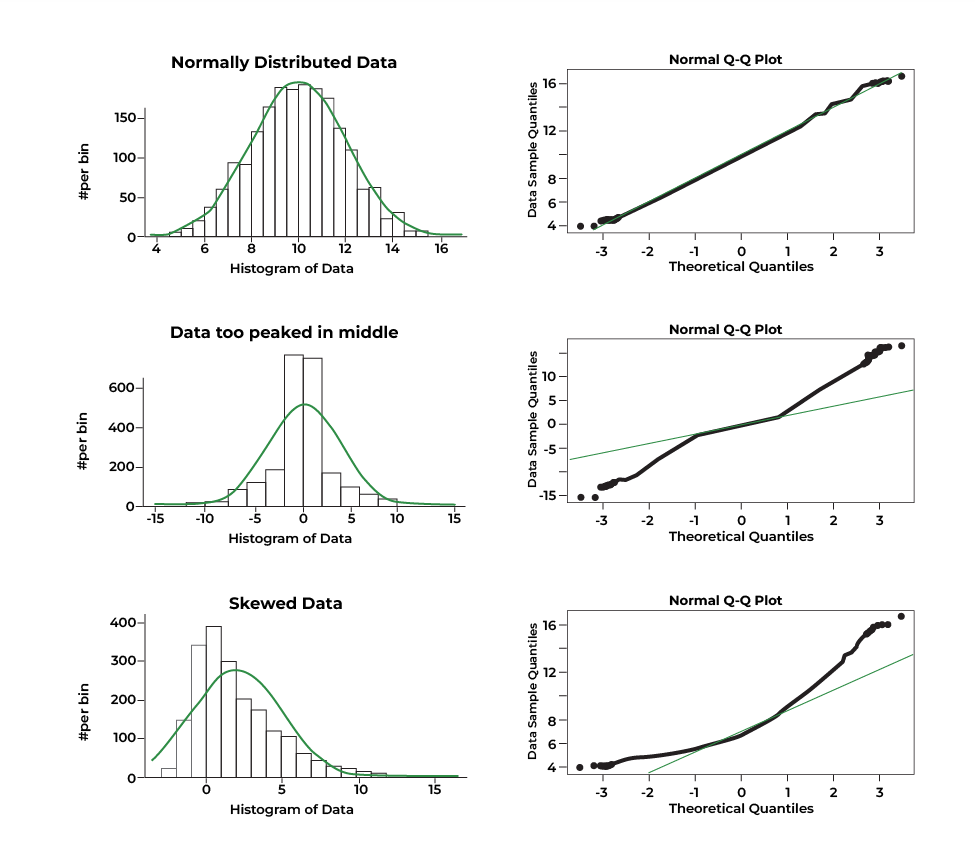
• The first row shows a normally distributed dataset, as evidenced by the bell-shaped histogram and the points falling close to a straight line in the Q-Q plot.

• The second row shows a dataset that is too peaked in the middle, indicating a deviation from normality.

• The third row shows a skewed dataset, also indicating a deviation from normality.

Therefore, the image demonstrates how different distributions can affect the assumption of Multivariate Normality.

4. Homoscedasticity of Residuals in Linear Regression

Homoscedasticity is one of the key assumptions of linear regression, which asserts that the residuals (the differences between observed and predicted values) should have a constant variance across all levels of the independent variable(s). In simpler terms, it means that the spread of the errors should be relatively uniform, regardless of the value of the predictor.

When the residuals maintain constant variance, the model is said to be homoscedastic. Conversely, when the variance of the residuals changes with the level of the independent variable, we refer to this phenomenon as heteroscedasticity.

Heteroscedasticity can lead to several issues:

• Inefficient Estimates: The estimates of the coefficients may not be the best linear unbiased estimators (BLUE), meaning that they could be less accurate than they should be.

• Impact on Hypothesis Testing: Standard errors can become biased, leading to unreliable significance tests and confidence intervals.

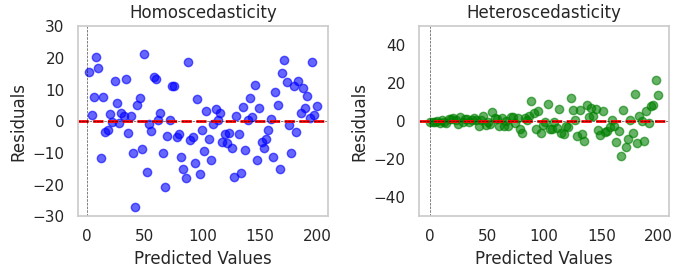
• Left plot (Homoscedasticity): The residuals are scattered evenly around the horizontal line at zero, indicating a constant variance.

• Right plot (Heteroscedasticity): The residuals are not evenly scattered. There is a clear pattern of increasing variance as the predicted values increase, indicating heteroscedasticity.

🔹 8. Polynomial Regression

Polynomial Regression extends linear regression by introducing higher-degree terms.

Equation:

Use Case: Modeling nonlinear relationships.

🔹 9. ML Project Pipeline

1. Problem Definition

2. Data Collection

3. Data Cleaning

4. Exploratory Data Analysis (EDA)

5. Data Splits

6. Model Selection

7. Training & Evaluation

8. Model Testing

9. Model Evaluation

10. Hyperparameter Tuning

11. Deployment

12. Monitoring

🔹 10. Data Standardization

Standardization scales features to have zero mean and unit variance:

Helps in improving model performance, especially for gradient-based algorithms.

🔹 11. Fit_transform vs Transform

• fit_transform() → used on training data; computes mean & std and applies scaling.

• transform() → used on test data using mean & std computed from training data.

from sklearn.preprocessing import StandardScaler
scaler = StandardScaler()
X_train = scaler.fit_transform(X_train)
X_test = scaler.transform(X_test)

🔹 12. MAE vs MSE

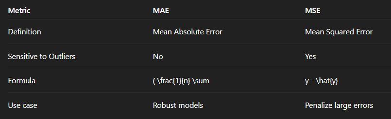
🔹 13. R-square and Adjusted R-square

R² (Coefficient of Determination): Proportion of variance explained by the model.

• R-squared or the coefficient of determination, is the statistical measure of the variance of the regression (best fit) line from the actual data points. In a generalized linear regression model the model accuracy ranging from 75 - 95% is considered as a good prediction model, whereas 100% accuracy means overfitting.

• R-squared values range from 0 to 1:

  • An R-squared of 0 indicates that the model explains none of the variability of the dependent variable.

  • An R-squared of 1 indicates that the model explains all the variability of the dependent variable.

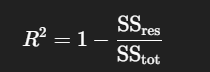
For example, an R-squared value of 0.85 suggests that 85% of the variance in the dependent variable can be explained by the independent variables in the model.

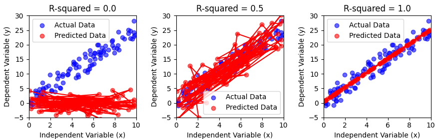
• R-squared = 0.0: The predicted points are randomly scattered, indicating the model has no predictive power. The independent variable (x) does not explain any variation in the dependent variable (y).

• R-squared = 0.5: The predicted points show a moderate relationship with the actual data. The model explains some variation in y, but a lot remains unexplained.

• R-squared = 1.0: The predicted points perfectly align with the actual data, indicating a perfect fit. The independent variable explains all the variation in y.

Adjusted R²: Adjusts R² for the number of features to avoid overfitting.

• Adjusted R-squared is a performance metrics which can be termed as a more refined version of R-squared which priorities the input features that correlates with the target variable. It takes into account the number of predictors in the model and whether they are significant. While R-squared always increases when more predictors are added, Adjusted R-squared increases only if the new predictors genuinely improve the model. It prevents overfitting by balancing the model’s performance with its complexity. Formula for Adjusted R-squared is:

  

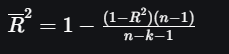
• n = number of data points (observations)

• k = number of predictors (features)

A higher Adjusted R-squared indicates that the model fits the data well without including unnecessary predictors, suggesting that the chosen features are meaningful and contribute to explaining the variability in the dependent variable. On the other hand, a lower or negative Adjusted R-squared suggests that adding more predictors does not improve the model’s performance and may even harm it. This occurs when extra predictors add noise rather than value.

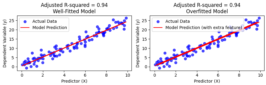
Both models have the same adjusted R-squared value of 0.94 explaining significant variation in the dependent variable:

• Well-Fitted Model: The predicted line aligns well with the data, capturing the true relationship between X and y.

• Overfitted Model: Though it has a high Adjusted R-squared (0.94), the line is too wiggly, indicating the model is overfitting by learning noise instead of the true pattern.

Key Differences Between R-squared and Adjusted R-squared

1. The value of R-squared increases when we increase an independent factor , whereas the value of Adjusted R-square increases only when the independent factor is necessary for the dependent factor.

2. The value of R-square can not be negative, whereas the value of Adjusted R-squared value can be negative.

3. R-squared favors complex models without penalizing for irrelevant predictors, while Adjusted R-squared penalizes unnecessary predictors, promoting simpler, more generalizable models.

Which is Better to Use R or R-squared?

When deciding whether to use R or R-squared in statistical analysis, it depends on what you want to convey:

Use R when you want to describe the strength and direction of a linear relationship. It ranges from -1 to 1, where values closer to -1 or 1 indicate a stronger relationship. Use R-squared when you want to understand how well your model explains the variability of the response data around its mean. It is particularly useful in assessing the goodness-of-fit of a regression model.

• R provides information about correlation strength and direction, while R-squared provides insight into how much variance is explained by the model.

• R is more intuitive for understanding relationships in simple regression, whereas R-squared is more informative for evaluating model fit, especially in multiple regression contexts.

🔹 14. Bias-Variance Tradeoff, Overfitting & Underfitting

• High Bias → Underfitting

• High Variance → Overfitting

Tradeoff is finding the sweet spot between bias and variance for better generalization.

1. Overfitting in Machine Learning

Overfitting happens when a model learns too much from the training data, including details that don’t matter (like noise or outliers).

• For example, imagine fitting a very complicated curve to a set of points. The curve will go through every point, but it won’t represent the actual pattern.

• As a result, the model works great on training data but fails when tested on new data.

Overfitting models are like students who memorize answers instead of understanding the topic. They do well in practice tests (training) but struggle in real exams (testing).

Reasons for Overfitting:

1.  High variance and low bias.

2. The model is too complex.

3. The size of the training data.

2. Underfitting in Machine Learning

Underfitting is the opposite of overfitting. It happens when a model is too simple to capture what’s going on in the data.

• For example, imagine drawing a straight line to fit points that actually follow a curve. The line misses most of the pattern.

• In this case, the model doesn’t work well on either the training or testing data.

Underfitting models are like students who don’t study enough. They don’t do well in practice tests or real exams. Note: The underfitting model has High bias and low variance.

Reasons for Underfitting:

1. The model is too simple, So it may be not capable to represent the complexities in the data.

2. The input features which is used to train the model is not the adequate representations of underlying factors influencing the target variable.

3. The size of the training dataset used is not enough.

4. Excessive regularization are used to prevent the overfitting, which constraint the model to capture the data well.

5. Features are not scaled.

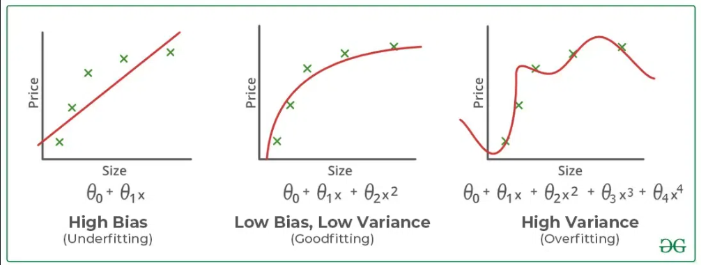
• Underfitting : Straight line trying to fit a curved dataset but cannot capture the data's patterns, leading to poor performance on both training and test sets.

• Overfitting: A squiggly curve passing through all training points, failing to generalize performing well on training data but poorly on test data.

• Appropriate Fitting: Curve that follows the data trend without overcomplicating to capture the true patterns in the data.

How to Address Overfitting and Underfitting?

Techniques to Reduce Underfitting

1. Increase model complexity.

2. Increase the number of features, performing feature engineering.

3. Remove noise from the data.

4. Increase the number of epochs or increase the duration of training to get better results.

Techniques to Reduce Overfitting

1. Improving the quality of training data reduces overfitting by focusing on meaningful patterns, mitigate the risk of fitting the noise or irrelevant features.

2. Increase the training data can improve the model's ability to generalize to unseen data and reduce the likelihood of overfitting.

3. Reduce model complexity.

4. Early stopping during the training phase (have an eye over the loss over the training period as soon as loss begins to increase stop training).

5. Ridge Regularization and Lasso Regularization.

6. Use dropout for neural networks to tackle overfitting.

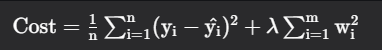
🔹 15. Regularization Techniques

Used to prevent overfitting by adding penalty terms.

Regularization is an important technique in machine learning that helps to improve model accuracy by preventing overfitting which happens when a model learns the training data too well including noise and outliers and perform poor on new data. By adding a penalty for complexity it helps simpler models to perform better on new data. In this article, we will see main types of regularization i.e Lasso, Ridge and Elastic Net and see how they help to build more reliable models.

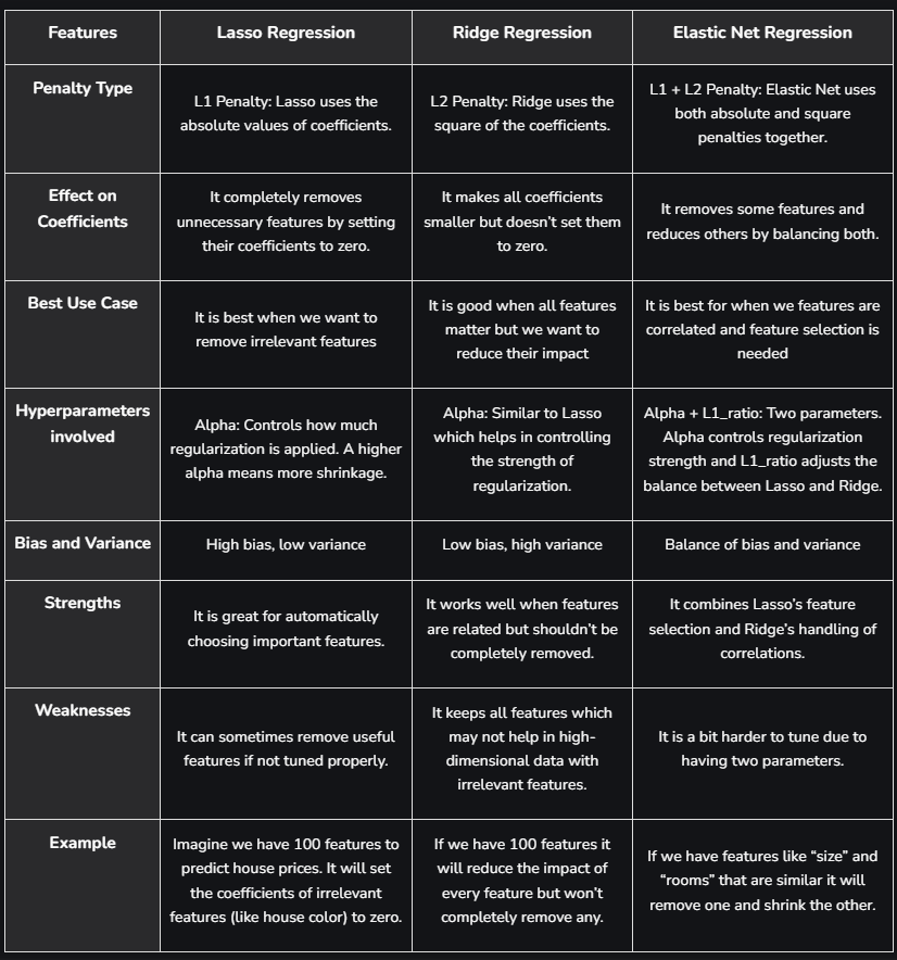
L1 Regularization (Lasso): Shrinks some coefficients to zero → feature selection.

• A regression model which uses the L1 Regularization technique is called LASSO (Least Absolute Shrinkage and Selection Operator) regression. It adds the absolute value of magnitude of the coefficient as a penalty term to the loss function(L). This penalty can shrink some coefficients to zero which helps in selecting only the important features and ignoring the less important ones.

where

• mm - Number of Features

• nn- Number of Examples

• yi- Actual Target Value

• y^i- Predicted Target Value

L2 Regularization (Ridge): Shrinks coefficients but doesn't make them exactly zero.

A regression model that uses the L2 regularization technique is called Ridge regression. It adds the squared magnitude of the coefficient as a penalty term to the loss function(L). It handles multicollinearity by shrinking the coefficients of correlated features instead of eliminating them.

where,

• nn= Number of examples or data points

• mm = Number of features i.e predictor variables

• yi= Actual target value for the ithith example

• y^i = Predicted target value for the ithith example

• wi = Coefficients of the features

• λ= Regularization parameter that controls the strength of regularization

ElasticNet: Combines L1 and L2.

Elastic Net Regression is a combination of both L1 as well as L2 regularization. That shows that we add the absolute norm of the weights as well as the squared measure of the weights. With the help of an extra hyperparameter that controls the ratio of the L1 and L2 regularization.

where

• n = Number of examples (data points)

• m = Number of features (predictor variables)

• yi = Actual target value for the ithith example

• y^i = Predicted target value for the ithith example

• wi= Coefficients of the features

• λ= Regularization parameter that controls the strength of regularization

• α = Mixing parameter where 0 ≤ α ≤ 1 and α = 1 corresponds to Lasso (L1) regularization, α = 0 corresponds to Ridge (L2) regularization and Values between 0 and 1 provide a balance of both L1 and L2 regularization

📌 Important Questions for Practice

1. What is the intuition behind linear regression?

2. How does gradient descent work?

3. What is the role of learning rate?

4. What’s the difference between MSE and MAE?

5. What is the difference between loss function and cost function?

6. Why do we standardize data before training?

7. Explain R² and Adjusted R² with an example.

8. What are assumptions of linear regression and what if they are violated?

9. What is the difference between Lasso and Ridge regression?

10. What causes overfitting and how can we prevent it?

11. Why we are not doing fit_transform in the test set and let say if we do fit_transform in the set what will be the impact on the model result?

🔗 Conclusion

Understanding these foundational ML concepts is essential for building robust models and cracking ML interviews. Linear regression may seem simple but grasping its mathematical and practical aspects paves the way to mastering advanced algorithms.